My First Deep Learning Practice via Adopting Linear Regression Model
Environment Preparation.
Prepare Three Dependencies
# Pandas allow to read data set
$ pip install pandas
# scikit learn is Machine Learning Library for Regression
$ pip install -U scikit-learn
# matplotlib allows visualize model and data
$ brew install freetype
$ brew install libpng
$ git clone git://github.com/matplotlib/matplotlib.git
$ cd matplotlib/
$ python setup.py install
Here is a quicker way to get your preparation done
$ cat requirements.txt
matplotlib==1.5.1
numpy==1.11.0
pandas==0.18.0
scikit-learn==0.17.1
Then
Then
$ pip install -r requirements.txt
Prepare a python script to read the dedup dataset, learning with linear regression model and display in matplot visualization UI.
$ cat demo.py
#Data is labeled and We use Supervisor Approach
#Type of machine learning task will perform is called regression ( Linear Regression )
import pandas as pd
from sklearn import linear_model
import matplotlib.pyplot as plt
#read data
dataframe = pd.read_fwf('dedup_seq_var_1_17.txt')
x_values = dataframe[['dedup']]
y_values = dataframe[['time']]
#train model on data
body_reg = linear_model.LinearRegression()
body_reg.fit(x_values, y_values)
#visualize results
plt.scatter(x_values, y_values)
plt.plot(x_values, body_reg.predict(x_values))
#plt.interactive(True)
plt.show()
Prepare your dataset, e.g different dedup files (size) to compare with dedup ratio and dedup process time.
file_name
|
Dedup
|
Time
|
seq_377K.0.0
|
96.25409276
|
2512
|
seq_610K.0.0
|
96.76181481
|
1742
|
seq_987K.0.0
|
97.22268395
|
18379
|
seq_1597K.0.0
|
97.28971803
|
4174
|
seq_2584K.0.0
|
97.51585024
|
3796
|
seq_4181K.0.0
|
97.53909053
|
8360
|
seq_6765K.0.0
|
97.57731661
|
9649
|
seq_10946K.0.0
|
97.70243732
|
12128
|
seq_17711K.0.0
|
97.73371995
|
26217
|
seq_28657K.0.0
|
97.75899063
|
36044
|
seq_46368K.0.0
|
97.77537807
|
56288
|
seq_75025K.0.0
|
97.77286868
|
89911
|
seq_121393K.0.0
|
97.7728039
|
130598
|
seq_196418K.0.0
|
97.76114378
|
231925
|
seq_317811K.0.0
|
97.76875575
|
365581
|
seq_514229K.0.0
|
97.77152402
|
587564
|
seq_832040K.0.0
|
97.77271286
|
946887
|
Final Output Example
 |
| Linear Regression ( y = mx + b ) diagram when m = dedup ratio and b = time |
As the result
is linear when we use variable chunking with modulo 128K but when file size
larger then 196418K ( 196.418 MB ), then process time got exponential grow in
this case.
Double check with Linear Regression Equation via NumPy
$ cat ./demo.py
from numpy import *
# y = mx + b
# m is slope, b is y-intercept
# this is error equation for collecting the error during different iteration
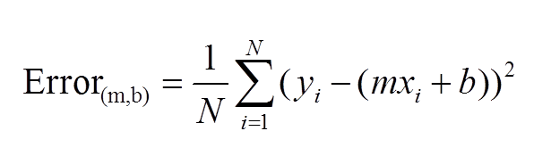
def compute_error_for_line_given_points(b, m, points):
#compute the distance from point to line and find the min which is best fit line for all the points
#y - y^2(mx+b) but we take sqare for y and summarize it and take average n
#initialize it at 0
totalError = 0
#for every points
for i in range(0, len(points)):
#get x value
x = points[i, 0]
#get y value
y = points[i, 1]
#get the difference, square it, add it to the total
totalError += (y - (m * x + b)) ** 2
#get the average
return totalError / float(len(points))
#gradient follows this partial derivative equation
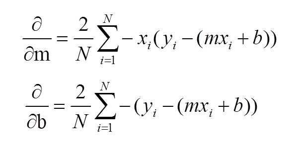
def step_gradient(b_current, m_current, points, learningRate):
#initial, starting points for gradients
b_gradient = 0
m_gradient = 0
N = float(len(points))
for i in range(0, len(points)):
x = points[i, 0]
y = points[i, 1]
#direction with respect to b and m
#computing partial derivatives of our error function ( partial derivative equations )
b_gradient += -(2/N) * (y - ((m_current * x) + b_current))
m_gradient += -(2/N) * x * (y - ((m_current * x) + b_current))
#update b and m values using partial derivatives
new_b = b_current - (learningRate * b_gradient)
new_m = m_current - (learningRate * m_gradient)
return [new_b, new_m]
def gradient_descent_runner(points, starting_b, starting_m, learning_rate, num_iterations):
#starting b and m
b = starting_b
m = starting_m
#gradient descent
for i in range(num_iterations):
#update b and m with the new more accurate b and m by performing
#this gradient step
b, m = step_gradient(b, m, array(points), learning_rate)
#once for loop finish, then return the ultimated b and m result
return [b, m]
def run():
#step 1 - collect data, two colums , colum 1: hours study (x), colum 2: test score (y)
points = genfromtxt("data.csv", delimiter=",")
#step 2 - define hyperparameters ( it's a balance )
#hyper-parameter 1: learning rate = how fast should our model converage
#converagence ( converage ) = means when you get the optimal results(model), the line of best fit. ( best answer )
#learning rate too low , get slow convergence, if too big, the error function might not decrease.
learning_rate = 0.0001
#hyper-parameter 2: equation ( slope formula ): y - mx + b
initial_b = 0 # initial y-intercept guess
initial_m = 0 # initial slope guess
#hyper=parameter 3: iteration
num_iterations = 10000
#Step 3 - train ML model
print "Starting gradient descent at b = {0}, m = {1}, error = {2}".format(initial_b, initial_m, compute_error_for_line_given_points(initial_b, initial_m, points))
print "Running..."
[b, m] = gradient_descent_runner(points, initial_b, initial_m, learning_rate, num_iterations)
print "After {0} iterations b = {1}, m = {2}, error = {3}".format(num_iterations, b, m, compute_error_for_line_given_points(b, m, points))
if __name__ == '__main__':
run()
$ cat data.csv
96.25409276,2512
96.76181481,1742
97.22268395,18379
97.28971803,4174
97.51585024,3796
97.53909053,8360
97.57731661,9649
97.70243732,12128
97.73371995,26217
97.75899063,36044
97.77537807,56288
97.77286868,89911
97.7728039,130598
97.76114378,231925
97.76875575,365581
97.77152402,587564
97.77271286,946887
$ python demo.py
Starting gradient descent at b = 0, m = 0, error = 85896989939.5
Running...
After 1000 iterations b = -58.9851802482, m = 1531.65706095, error = 63605989287.1
$ cat data.csv
96.25409276,2512
96.76181481,1742
97.22268395,18379
97.28971803,4174
97.51585024,3796
97.53909053,8360
97.57731661,9649
97.70243732,12128
97.73371995,26217
97.75899063,36044
97.77537807,56288
97.77286868,89911
97.7728039,130598
$ python demo.py
Starting gradient descent at b = 0, m = 0, error = 2383362378.46
Running...
After 1000 iterations b = -13.93366184, m = 316.652164833, error = 1432258731.3
The interesting thing is if we remove file larger than seq_10946K in data set, we got lowest error as result.
$ cat data.csv
96.25409276,2512
96.76181481,1742
97.22268395,18379
97.28971803,4174
97.51585024,3796
97.53909053,8360
97.57731661,9649
$ python demo.py
Starting gradient descent at b = 0, m = 0, error = 77422434.5714
Running...
After 1000 iterations b = -1.28801270757, m = 71.5887947793, error = 29053565.2771
In sum, when we use variable chunk and modulo 128K ( 0.85 * 128K ( min ) ~ 2 * 128K ( max ) ) as chunking boundary are kinds of follow linear pattern when file is smaller than 196.418MB. However, when file size larger than 196.418MB, the process time is not follow the linear patter compare with dedup ratio and might be obviously become explanation growing patten. Moreover, when we use variable chunking with mod 128K, against with different file size, when file size under 10946K, then we might keep lowest error rate in this data set.
Extra Bonus:
Here is the practice I was doing for 3 parameters in linear regression. Regarding the juypter note, you can easy to track down the code and generate those linear graphics.
https://github.com/chianingwang/DeepLearningPractice/blob/master/linear_regression/linear-regression_sklearn/linear_regression.ipynb


不要害怕犯錯。只有當你停止犯錯的時候,才需要警惕。因為這代表著你已經不再學習,或停止進步。
Reference:
https://github.com/chianingwang/DeepLearningPractice/tree/master/linear_regression
https://github.com/llSourcell/linear_regression_demo
https://github.com/llSourcell/linear_regression_live
Extra Bonus:
Here is the practice I was doing for 3 parameters in linear regression. Regarding the juypter note, you can easy to track down the code and generate those linear graphics.
https://github.com/chianingwang/DeepLearningPractice/blob/master/linear_regression/linear-regression_sklearn/linear_regression.ipynb
Here are leverage 2D and predict 2D

Here are the 3D plots diagram


Here are the prediction base on the existing data.


不要害怕犯錯。只有當你停止犯錯的時候,才需要警惕。因為這代表著你已經不再學習,或停止進步。
Don't be afraid to make mistakes. The only time you should be worried is when you stopped making mistakes; it only means that you've stopped learning or making progress.
進擊的鼓手 (Whiplash), 2014
Reference:
https://github.com/chianingwang/DeepLearningPractice/tree/master/linear_regression
https://github.com/llSourcell/linear_regression_demo
https://github.com/llSourcell/linear_regression_live